The explosive growth of open-source model repositories has created a Model Jungle, where checkpoints are frequently shared without adequate documentation or metadata. While weight-space learning offers a pathway to identify and analyze these models directly from their parameters, processing full-scale weights is computationally prohibitive. Probing-based methods have emerged as a lightweight alternative, extracting permutation-equivariant representations via learnable probe vectors. However, existing probing methods are limited by a single-view design: they capture first-order structures but fail to encode the rich, higher-order correlation patterns inherent in row–column interactions. To bridge this gap, we introduce MVProbe, a multi-perspective probing framework that synthesizes first-order signals with interaction-aware (Gram-based) views. Our approach is theoretically grounded; we analyze the scaling laws of different probing orders to derive a principled standardization and fusion strategy that ensures balanced contributions from all branches. On the Model Jungle benchmark, MVProbe consistently outperforms the state-of-the-art ProbeX across diverse architectures, including ResNet, SupViT, MAE, and DINO.
Existing single-direction probes summarize a weight matrix \(\mathbf{X}\in\mathbb{R}^{m\times n}\) by a single first-order projection \(\mathbf{X}\mathbf{u}\). Such projections are inherently ambiguous: distinct weight matrices can produce identical probe responses, collapsing them to the same representation. They also miss higher-order structure such as the row–column correlations encoded in the Gram matrices \(\mathbf{X}\mathbf{X}^{\top}\) and \(\mathbf{X}^{\top}\mathbf{X}\).
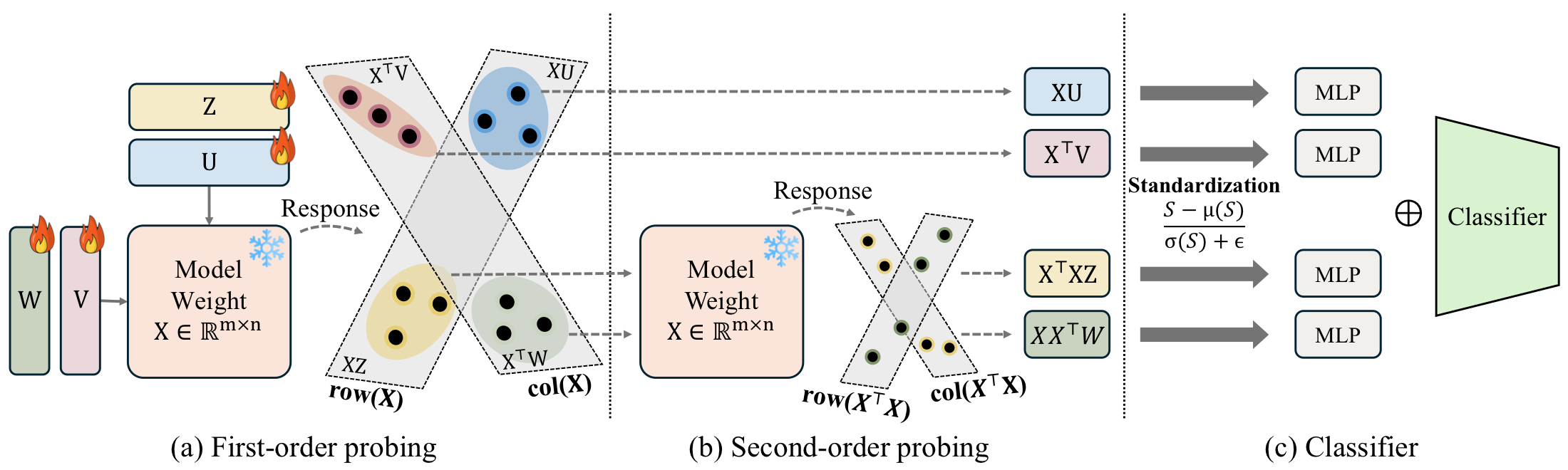
MVProbe addresses this with four complementary branches. First-order branches use learnable probe matrices \(\mathbf{U},\mathbf{V}\) and produce \(\mathbf{XU}\) and \(\mathbf{X}^{\top}\mathbf{V}\) — direct row/column projections. Second-order (kernel) branches use probe matrices \(\mathbf{W},\mathbf{Z}\) and apply the Gram operators to produce \(\mathbf{XX}^{\top}\mathbf{W}\) and \(\mathbf{X}^{\top}\mathbf{XZ}\), which encode pairwise similarity structure between output and input neurons, respectively. Each branch is followed by per-sample standardization, a branch-specific MLP, and feature concatenation; a shared encoder and classifier head complete the model.
We motivate this design from two perspectives. From kernel methods, Gram matrices encode pairwise similarity that first-order projections cannot capture. From landmark-based representations in manifold learning, the four probe matrices act as learned reference directions and kernel-space landmarks that together coordinate the geometry of the weight matrix.
Conceptual illustration of Theorem 1. With the same probe matrix \(\mathbf{U}\), two distinct weight matrices \(\mathbf{X}_1\) and \(\mathbf{X}_2\) may collapse to the same first-order probe response \(\mathbf{XU}\), making them indistinguishable. Passing them through the Gram operator \(\mathbf{X}^{\top}\mathbf{X}\) once more (second-order probing) separates them again — recovering the information lost to a single linear projection.
Theorem 1 — Expressiveness of Second-Order Probes
Let \(\mathbf{U}\in\mathbb{R}^{n\times r}\) be a probe matrix with \(\mathrm{rank}(\mathbf{U})=r<n\), and define the first- and second-order features \(\Phi_1(\mathbf{X}) := \mathbf{X}\mathbf{U}\) and \(\Phi_2(\mathbf{X}) := (\mathbf{X}^{\top}\mathbf{X})\mathbf{U}\). Then there exist distinct \(\mathbf{X}_1\neq\mathbf{X}_2\) with \(\Phi_1(\mathbf{X}_1)=\Phi_1(\mathbf{X}_2)\) but \(\Phi_2(\mathbf{X}_1)\neq\Phi_2(\mathbf{X}_2)\). Consequently, when \(r<n\), adding second-order branches separates weight matrices that are indistinguishable to first-order probing alone.
Theorem 2 — Transpose-Complement Non-Redundancy
Let \(\mathbf{U}\in\mathbb{R}^{n\times r}\) and \(\mathbf{V}\in\mathbb{R}^{m\times r}\) be probe matrices with \(\mathrm{rank}(\mathbf{U})=r<n\). There exist distinct \(\mathbf{X}_1,\mathbf{X}_2\) such that \(\mathbf{X}_1\mathbf{U}=\mathbf{X}_2\mathbf{U}\) but \(\mathbf{X}_1^{\top}\mathbf{V}\neq\mathbf{X}_2^{\top}\mathbf{V}\). Hence the column-side branch \(\mathbf{X}^{\top}\mathbf{V}\) supplies information that is not recoverable from the row-side branch \(\mathbf{X}\mathbf{U}\) alone — both first-order branches are needed.
Theorem 3 — Scale Imbalance & Standardization
For \(\mathbf{X}\) with i.i.d. \(\mathcal{N}(0,\sigma^2)\) entries and unit-norm probe columns, the expected scale ratio between the second- and first-order responses is \(\mathbb{E}\!\left[\|\mathbf{S}^{(2)}\|_F^2\right]/ \mathbb{E}\!\left[\|\mathbf{S}^{(1)}\|_F^2\right] = \tfrac{n(n+m+1)}{m}\sigma^2 = \mathcal{O}(n\sigma^2)\), so naive concatenation is dominated by the second-order branch. Per-sample standardization yields \(\|\tilde{\mathbf{S}}\|_F^2 = mr\) regardless of order, equalizing branch contributions and motivating the standardization block in MVProbe.
MVProbe vs ProbeX on the Model Jungle benchmark.
Discriminative — fine-tune class identification
Generative — Stable Diffusion LoRA identification
Accuracy (%), mean±std over seeds 1–5 on the Model Jungle benchmark.
| Method | ResNet | SupViT | MAE | DINO |
|---|---|---|---|---|
| StatNN | 55.20 | 55.80 | 54.83 | 55.69 |
| ProbeGen | 78.27 | 78.48 | 70.68 | 61.26 |
| ProbeX | 81.61±1.29 | 88.08±0.39 | 77.11±0.14 | 72.54±0.18 |
| ProbeX (×4) | 87.16±0.26 | 90.33±0.31 | 77.26±0.12 | 73.25±0.21 |
| MVProbe (Ours) | 92.24±0.25 | 92.33±0.37 | 81.62±0.15 | 78.29±0.31 |
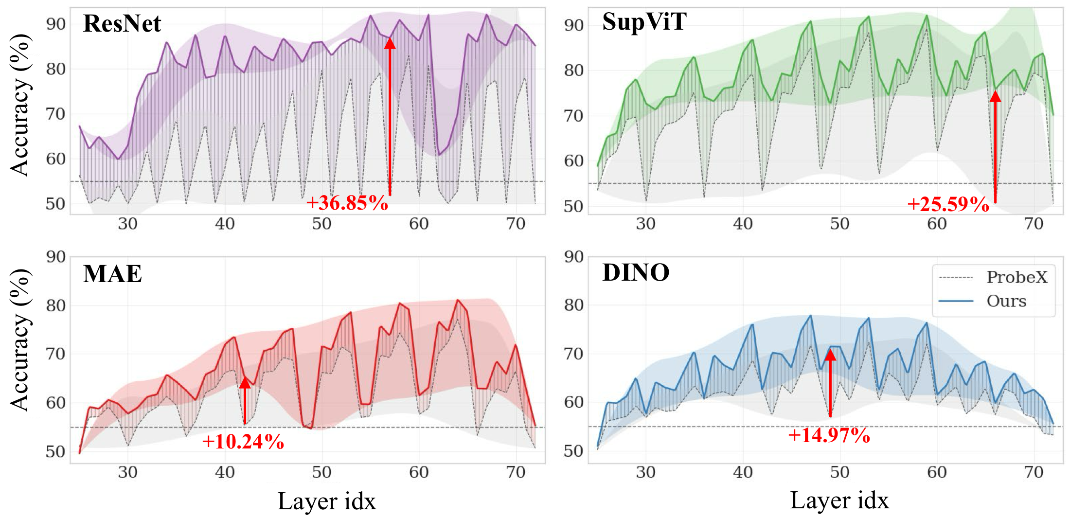
Layer-wise performance comparison. MVProbe (solid lines) vs. ProbeX (dashed lines) across all layers. Shaded bands indicate the performance volatility. MVProbe maintains higher accuracy across most layers and shows less sensitivity to layer selection.
In-distribution and zero-shot accuracy on SD_200 and SD_1k LoRA adapters (mean±std over seeds 1–5, layer 46).
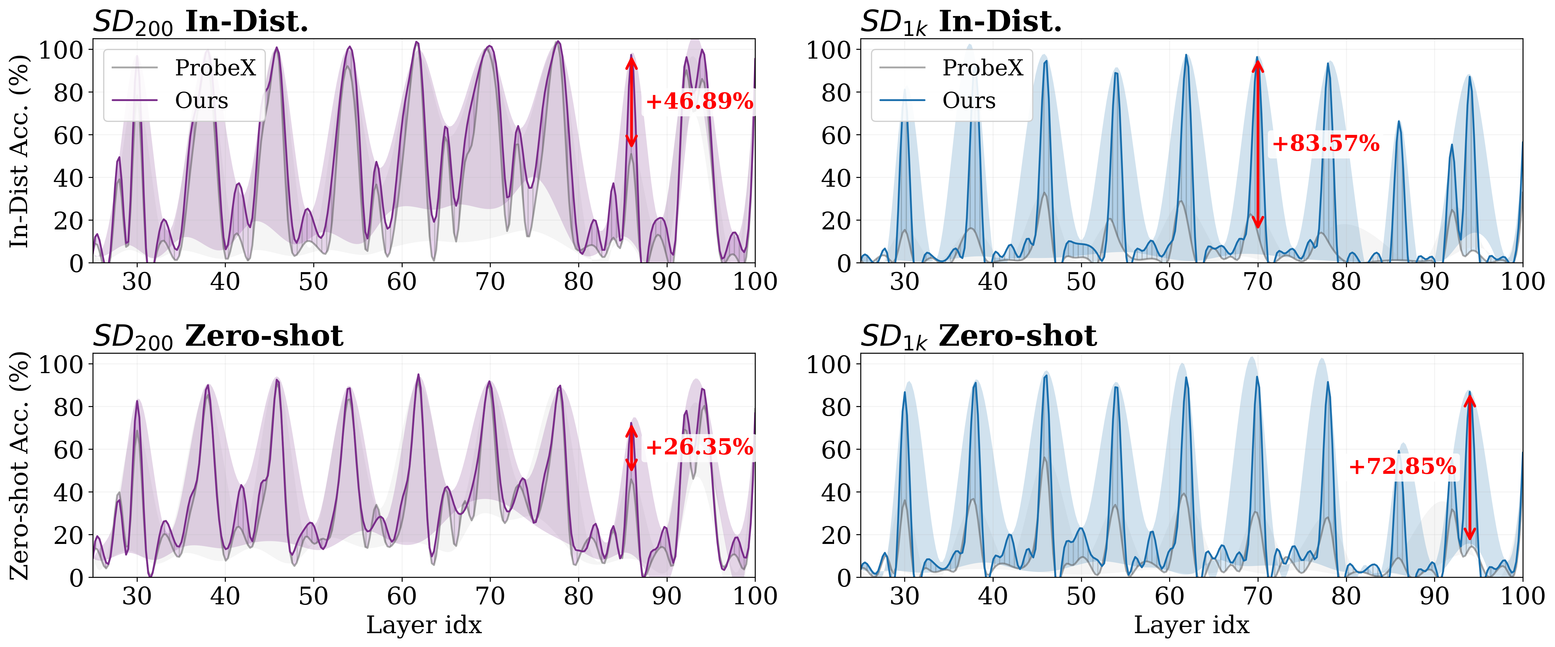
Layer-wise performance on SD LoRA. MVProbe (solid lines) vs. ProbeX (dashed lines) across all layers on \(\text{SD}_{200}\) and \(\text{SD}_{1k}\) (In-Distribution and Zero-shot). Shaded bands indicate per-layer volatility; red arrows mark the largest gains.
| Method | In-Distribution Acc | Zero-shot Acc |
|---|---|---|
| ProbeX | 98.48±0.48 | 94.01±0.77 |
| ProbeX (×4) | 97.72±0.50 | 93.53±1.99 |
| MVProbe (Ours) | 99.80±0.00 | 95.53±0.65 |
| Method | In-Distribution Acc | Zero-shot Acc |
|---|---|---|
| ProbeX | 35.75±2.44 | 52.42±2.48 |
| ProbeX (×4) | 32.46±3.08 | 51.14±3.88 |
| MVProbe (Ours) | 97.88±0.37 | 97.96±0.29 |